The curious case of Google's AlloyDB

Google launched AlloyDB in 2022. They claimed it is fully compatible with PostgreSQL. Can be up to 100 times faster for analytical queries than vanilla Postgres. Four years later, I haven't personally seen it gain significant traction. But it comes in discussions. When people ask me what AlloyDB actually is, I was able to pin point the features, but wasn't really sure what it delivers.

Over the past 12 months, I’ve evaluated AlloyDB. This article shares my key findings. I tried to keep it as objective as the topic allows, and where it isn't, the text says so. I won't pretend to be objective about the verdict. It depends less on one feature and more on where compatibility ends. And as it goes, "it depends" a lot on your workload and needs.

Let's start with the first claim. What does "fully compatible" mean? In this case it covers the wire protocol. Your psql connects, ORMs work, migration means changing connection string and you are done. What it does not cover is nearly everything you know about the Postgres storage internals and query executor. The 8KB pages that define storage layout for vanilla engine, are no longer the durable representation of your data. The WAL is no longer a recovery mechanism. It becomes the database. VACUUM is there, but runs inside storage layer you don't know and and schedule you can't control. And the tuning options differ from what you are be used to.

This creates the curious case. The compatibility claim is true, and the engineering behind AlloyDB backs it up. It's just narrower than the word "fully" migth suggest. AlloyDB is a different database behind the PostgreSQL protocol.

AlloyDB’s compatibility claim holds at the wire protocol, but the underlying engine diverges immediately at the storage layer.

What I'd verify before betting a migration on it:

• Whether your extensions survive the move. The allowlist differs between managed AlloyDB and Omni in ways you won't guess (plv8 and postgis trade places); timescaledb and pgrx are on neither.
• Whether the columnar store is actually resident before you trust a benchmark number, yours or mine. It can be enabled and silently empty.
• The read pool's economics for your read shape. Bursty business-hours reads and flat around-the-clock reads land on opposite sides of the break-even.
• Write contention at your scale. My own run inverted between SF10 and SF100, and not in the direction the pitch suggests.
• ScaNN recall at your vector count.

The log is the database

In standard PostgreSQL the query engine and the storage engine run as a single process, and that process owns its storage. It writes 8KB pages to disk and writes WAL records so that the system can reconstruct those pages after a crash. The pages hold the data, the log is there to repair them, and under normal operation the compute node pays for both.

AlloyDB inverts this. The compute node never writes full database pages to durable storage. Instead, it sends Write-Ahead Log (WAL) records to a distributed storage layer built on top of Colossus, Google's cluster file system. In this storage layer, a dedicated Log Processing Service (LPS) processes log records. It updates database pages asynchronously. When processing queries, the compute node fetches these pages as needed into its memory buffer pool. It also utilizes an ultra-fast local SSD block cache to cut reads from durable storage and accelerate page retrieval. Ultimately, the durable representation of your data is the log itself, and the data pages are derived from it without interruption.

This format is proprietary and not open for independent inspection. In contrast, PostgreSQL's on-disk format is something I typically examine byte by byte here on the blog. The account that follows therefore describes the architecture as Google documents it.

Five consequences follow; Google's marketing covers four of them.

Failover stops being a replay problem. In standard PostgreSQL, a promoted standby needs to finish replaying WAL before it can accept writes. The time this takes depends on how far behind it was. In AlloyDB there is no deviation to replay, because the storage is shared. A replacement compute node attaches to the same storage layer and picks up where the old one left off.

Read replicas are no longer copies. AlloyDB's "read pool" nodes are extra compute nodes attached to the same distributed storage as the primary. They still consume a log stream, and still flush and replay it, but they don't depend on replaying it to access the data.

Storage management shifts to Google too. As the storage layer grows on its own, issues like resizing windows and disk-full incidents disappear.

The write path drops full-page writes. Standard PostgreSQL protects against torn pages. It writes the full 8KB page into the WAL the first time it’s accessed after each checkpoint. full_page_writes is on by default for a good reason. It’s a well-known source of WAL volume. When a workload has small scattered updates, it can use more log space for full-page images than for the row changes themselves. AlloyDB never takes on this overhead. The storage layer replays log records into pages and protects against torn pages. So, the compute node doesn't checkpoint or send a full-page image. It only ships change records.

The fifth consequence is the one the marketing leaves out. You can no longer look at your own storage. There is no pageinspect equivalent for AlloyDB's durable format. You can check the buffer pool, which holds pages in the compute-node RAM. However, the format used is proprietary and unclear. If you've ever walked through MVCC headers byte by byte to solve a bloat issue or check what an UPDATE did, you can’t do that now. For many users this is an acceptable trade: they lose page-level visibility they probably never exercised and gain a managed storage layer.

Vacuum, rescheduled

Google's marketing barely mentions the consequence I went looking for first. VACUUM is a common topic for Postgres user and frequently covered on this blog. We’ve discussed everything from the lie in its name to what it does page by page. My first question was: what happens to it when storage moves off the compute node?

In standard PostgreSQL, VACUUM is the compute node's burden. Dead tuples build up in heap pages. Autovacuum workers scan the heap, remove them, and update the visibility map. They also compete with your queries for I/O during this process.

A whole subculture revolves around this:

• autovacuum_vacuum_scale_factor
• Cost-delay tuning
• Monitoring pg_stat_user_tables.n_dead_tup
• The issue of a long-running transaction that held back the xmin horizon, causing a table to double in size.

Going in, I expected vacuum to be the thing the storage layer absorbed. If the log is the database and pages are materialized on Google's side, dead tuples should be Google's problem. The stats say otherwise. The compute node uses the standard PostgreSQL executor with a standard buffer pool. So, UPDATE and DELETE leave dead tuples in the heap pages that the node reads. The tuples need pruning. The visibility map and free space map must be maintained. Also, rows need to be frozen before wraparound. That work still runs on the compute node. The storage layer sees every log record. It maintains versions of the blocks created from the log. Some cleanup happens outside the compute node, but the compute-side job remains unchanged. What Google actually replaced is the scheduler.

AlloyDB's adaptive autovacuum changes community autovacuum's fixed thresholds. It features a smart controller that boosts worker count when idle and reduces it when busy. This approach targets large table fragments instead of whole tables. It also slows down transaction-ID use if a wraparound horizon is near. Plus, it spots problems that block vacuum progress, like long-running transactions and orphaned prepared transactions. If a backend's XID age crosses a set limit, it logs a warning. That last part only diagnoses the problem. The benchmark below checks this: if the compute node still vacuums, then autovacuum_count should increase. Also, n_dead_tup should show a saw-tooth pattern.

This is verifiable from the outside, and you should verify it. Run a workload with many updates, like pgbench's default mix. Aim for a few hundred TPS for one hour. Test standard PostgreSQL and AlloyDB. Then, we can compare the results.

SELECT relname, n_dead_tup, n_live_tup,
       autovacuum_count, last_autovacuum
FROM pg_stat_user_tables
WHERE relname = 'pgbench_accounts';

On standard PostgreSQL you'll watch n_dead_tup saw-tooth, climbing between autovacuum passes and dropping after each one. AlloyDB does the same. Churning a one-million-row table with full-table UPDATEs on AlloyDB makes n_dead_tup rise to one to three million, then it drops. Meanwhile, autovacuum_count increases with each pass, seven total in seven minutes. The identical workload on Cloud SQL produces the same shape and seven passes. There is no flatline and no vacuum-free steady state. The compute node is running autovacuum, exactly as the stock engine does, and what AlloyDB changed is when it runs, not whether. (Both time series are in the repo.)

Managed AlloyDB supports pg_squeeze with the alloydb.enable_pg_squeeze flag. This means that when bloat builds up, you can perform an online, low-lock rebuild. It works like pg_repack in stock PostgreSQL, so no VACUUM FULL exclusive lock is needed.

Operationally this is a genuine win with one string attached. The win is that a recurring production failure mode (an instance accumulating vacuum debt faster than its autovacuum can clear it) is off your pager. The standard PostgreSQL vacuum rules now work differently or not at all. Any monitoring based on dead-tuple counts and autovacuum timing is tracking a process that Google controls. Alert thresholds calibrated against community autovacuum's fixed scale factors will fire on a schedule that no longer means what they were tuned for.

The in-memory columnar store

PostgreSQL stores rows. Every heap page packs complete tuples, all columns of a row adjacent on the page. For OLTP this is the right call, since fetching a row is one page read. For analytics it is the wrong one. Computing SUM(l_extendedprice * (1 - l_discount)) for 60 million lineitem rows requires reading all 60 million full 16-column tuples. However, only two columns are needed for the calculation. The buffer numbers in your EXPLAIN output tell that story every time.

AlloyDB uses an in-memory columnar store. This is a special memory area next to the buffer pool. It keeps certain columns from specific tables in columnar format. Plus, it supports vectorized execution. It is not a separate analytical database; there is no ETL, no second cluster, no sync job to babysit. The planner sees it as another access path. It picks between heap scan and columnar scan based on cost, just like it decides between sequential scan and index.

The columnar engine is not an extension. It is compiled into the AlloyDB binary; you cannot install it on a standard PostgreSQL installation, and you cannot remove it from AlloyDB.

The engine is observable through g_columnar_-namespaced relations. This is what the store held during the scale-factor-100 run, after the columns the query set touches were pinned (the full per-column dump is in the repo):

-- What's resident in the columnar store, by table
SELECT relation_name, count(*) AS columns, pg_size_pretty(sum(size_in_bytes))
FROM g_columnar_columns
GROUP BY relation_name ORDER BY sum(size_in_bytes) DESC;

 relation_name | columns | pg_size_pretty
---------------+---------+----------------
 lineitem      |      13 | 25 GB
 orders        |       6 | 5289 MB
 part          |       2 | 172 MB
 customer      |       2 | 129 MB
 supplier      |       2 | 8796 kB
 nation        |       2 | 954 bytes
 region        |       1 | 417 bytes

Population can happen automatically. A background process looks at query patterns to decide which columns need memory. It can also be done explicitly.

SELECT google_columnar_engine_add(
  'lineitem',
  'l_quantity,l_extendedprice,l_discount,l_shipdate,l_returnflag,l_linestatus'
);

Automatic population has a failure mode worth knowing, because it fails quietly, and I found it the hard way. The recommendation function uses observed columnar query history to decide what to cache. On a newly enabled engine or immediately after a restart, that history is empty, so the function may recommend nothing. The store stays empty, every plan falls back to a heap scan, and the queries run at full row-store speed with no error and no warning. The columnar engine is on, and it is doing nothing. The tell shows an empty g_columnar_columns and a Seq Scan, instead of the expected Custom Scan (columnar scan). Explicit google_columnar_engine_add sidesteps it. Either way, verify the columns are resident before you trust a number. I didn't on one of the early SF100 runs, and that run measured nothing.

When the planner picks the columnar path, the plan says so, and the buffer numbers explain why it's faster. Here is TPC-H Q6, which is the revenue query. It performs a selective scan of the lineitem table, accessing four columns. This is tested at a scale factor of 100, with about 600 million rows, on AlloyDB Omni. The tests were done with the columnar store both off and on. Same box, same query. Trimmed to the lines that matter, with cost= estimates and the filter predicates elided. These are the p90 runs, while the table below reports medians. Full plans are in the repo.

Columnar off, the row store:

 Finalize Aggregate  (actual time=182546.439..182546.691 rows=1 loops=1)
   Buffers: shared hit=2560 read=11549743
   I/O Timings: shared read=814349.441
   ->  Gather  (actual time=182546.333..182546.679 rows=5 loops=1)
         Workers Planned: 4
         Workers Launched: 4
         ->  Partial Aggregate  (actual time=182545.107..182545.108 rows=1 loops=5)
               ->  Parallel Seq Scan on lineitem  (actual time=0.690..181854.379 rows=2284274 loops=5)
                     Rows Removed by Filter: 117723307
                     Buffers: shared hit=2560 read=11549743
                     I/O Timings: shared read=814349.441
 Execution Time: 182546.776 ms

Columnar on:

 Finalize Aggregate  (actual time=594.954..595.135 rows=1 loops=1)
   ->  Gather  (actual time=594.058..595.125 rows=5 loops=1)
         Workers Planned: 4
         Workers Launched: 4
         ->  Partial Aggregate  (actual time=592.583..592.585 rows=1 loops=5)
               ->  Parallel Append  (actual time=0.187..592.573 rows=564 loops=5)
                     ->  Parallel Custom Scan (columnar scan) on lineitem  (actual time=0.186..592.569 rows=564 loops=5)
                           Rows Removed by Columnar Filter: 117723307
                           Rows Aggregated by Columnar Scan: 500216
                           Columnar cache search mode: native
                     ->  Parallel Seq Scan on lineitem  (never executed)
 Execution Time: 595.220 ms

182 seconds to 0.6 seconds, a 307x drop on this run and 311x at the table's median below, and the two lines that carry it are Buffers: shared read=11549743 and I/O Timings: shared read=814349. The row store reads 11.5 million pages off disk, 814 seconds of I/O summed across four workers and the leader, to filter out about 51 of every 52 rows. The columnar scan reads no heap pages at all. Columnar cache search mode: native means it answered entirely from the in-memory store, and the Parallel Seq Scan on lineitem (never executed) branch underneath it is the proof: the planner kept a heap path available and never touched it. The mechanism is the elimination of I/O: a heap scan of a 16-column table reads whole pages containing complete rows, then discards the unneeded column values; the columnar scan never loads those bytes. At 600 million rows the row store no longer fits in the buffer pool, so that discarded work becomes disk work.

One caveat on this pair, because it is not a single-variable experiment. To hold those columns, C1 had about 31 GB of columnar store on top of its 16 GB buffer pool, while the row-store run got the 16 GB and nothing else. So this measures the engine and roughly three times more memory over the hot data together. The two cannot be cleanly separated, because making the hot set fit is the mechanism: the heap here is about 100 GB, so no buffer pool on a 64 GB box closes that gap. The SF10 comparison further down has no such confound.

Q6 is the best case, not the general one. Across the query set at scale factor 100, the same columnar store on the same box produced these results:

query	shape	row store	columnar	speedup
Q6	selective scan, few columns	182,517 ms	587 ms	311x
Q5	six-table join	242,559 ms	24,688 ms	9.8x
Q12	join plus date filter	201,411 ms	41,708 ms	4.8x
Q1	full-table numeric aggregate	186,377 ms	94,195 ms	2.0x
point lookup	single row by key	0.15 ms	0.11 ms	none

A selective scan that reads some columns and ignores most rows is very effective. A join is also quite beneficial. A full-table numeric aggregate is somewhat useful, as the math outweighs the I/O. The single-row lookup is the control. The planner takes the b-tree and the columnar store never enters the plan, exactly as it should. So "up to 100x" is a number for one query shape at one scale, not a general multiplier: Q6 clears it comfortably here, and nothing else in the set comes close.

Two queries are missing from that table, and the reasons are worth stating. Q14's row-store run never happened. It died with could not resize shared memory segment, which is my own provisioning and not a property of either engine, so there is no baseline to compare the columnar run against. Q18 did run on the row store, three times, at around 655 seconds each. But the columnar run was killed by a 300-second statement timeout, so the two sides never ran under the same limit and no speedup can honestly be derived from the pair. Both are withdrawn rather than reported. At SF10, where both finish cleanly, Q18 gains 1.14x, the smallest win in the set.

When it helps, when it doesn't, when it hurts

The columnar store accelerates one shape of query.

It helps for scan-heavy aggregations over large tables touching few columns. TPC-H Q1, Q6, and Q14 are the canonical shapes. The dashboard query that counts and sums everything. AlloyDB's main selling point is the HTAP case. It runs a reporting query on live operational data. This happens because no one built the warehouse.

It doesn't help with point lookups, where the planner correctly takes the b-tree and the columnar store never enters the picture. Single-row OLTP. On small tables, the same aggregation on lineitem subsets shows that columnar is slower than heap with 100K rows (31.6 ms vs 27.5 ms). Here, the store's overhead is more than the scan. Columnar pulls ahead at around 1M rows, gaining a 1.2x speedup. This advantage grows to 2x by 20M rows. The crossover is around a few hundred thousand rows. Below that, the heap stays in the buffer pool, so there’s nothing to gain. This is an in-memory result at SF10, so it measures the vectorization crossover; at scale, where the heap spills to disk, columnar pays off far sooner.

It can hurt write-heavy tables with pinned columns. The columnar store must match the heap. So, when writes happen, they invalidate columnar blocks. Then, background work repopulates those blocks. Pin the columns of a table taking a thousand INSERTs a second and the maintenance can cost more than the scans save. Google's auto-population is supposed to notice and back off; whether it does for your write pattern is something to verify, not assume. Measured at the low end it is cheap. Pinning lineitem's columns added about 1% to a one-million-row bulk load (the number is in The numbers below), and that cost scales with write rate.

The main question about the HTAP pitch is: can the columnar engine maintain OLTP throughput while an analytical scan runs on the same instance? I expected it to. Taking the scan's I/O off the table should free the machine for writes. It doesn't. At SF10 it is a wash.

Write throughput drops by about 13.5% during concurrent scans, whether reading from the heap or store. This happens because the scanned table is in memory. The issue is with compute contention, not I/O, and columnar structures don't help with that. Fair enough at that size, nothing to win.

At SF100, where the heap spills to disk, turning columnar on makes the contention worse (29% versus 16%). The mechanism and the full numbers are in The numbers below. For deployment, what it means is that the isolation has to come from a dedicated read pool node with its own CPUs, and it is paid for in visibility lag.

AlloyDB Omni: same name, different product

AlloyDB Omni is the downloadable AlloyDB, a container image you run on your own infrastructure (Kubernetes, a VM, your laptop).

docker pull google/alloydbomni:18   # or a specific tag like 18.1.1

One sign that Omni is a separate product is its timing. When managed AlloyDB hit PostgreSQL 18 (GA May 2026), the Omni Linux packages updated. However, the Docker Hub image lagged, staying at version 17 for a while. The release trains are separate. Check the tag you actually pull.

The AlloyDB compute layer includes several components. It has a columnar engine. This engine uses the same API and includes the google_columnar_engine_* relations. Also, it has the ScaNN vector index and updates to the AlloyDB planner.

What's not inside is everything in the first half of this article. Omni runs on standard PostgreSQL storage. Real 8KB pages on your filesystem, WAL as a recovery mechanism, ordinary autovacuum doing ordinary VACUUM work. Start an Omni container and check pg_settings. full_page_writes is on, and checkpoint_timeout is five minutes. This means the write path handles full-page images like stock PostgreSQL.

However, Omni doesn't inherit those write-path advantages. No disaggregated storage. No shared-storage read pools. Omni replicas are just plain streaming replication, with lag included. There’s no managed failover, so bring your own Patroni. The one storage-flavored feature that does come along is the ultra-fast SSD cache, and only as a knob. In Omni you point a disk cache at a local SSD and size it yourself; managed provisions and sizes it for you.

Managed AlloyDB and AlloyDB Omni are different in design but share the same query layer. Omni is much closer to a PostgreSQL fork with a columnar engine bolted in than to a portable version of the cloud product. That doesn't make it uninteresting; the columnar engine on your own hardware, without GCP, stands on its own. But if the storage-layer properties are what attracted you, Omni does not have them.

Omni is the clean benchmark platform for isolating the columnar engine's share of AlloyDB's analytical performance. It runs TPC-H tests with the engine off and then on. That pair is the two Omni columns in The numbers below, and it is the cleanest isolation in the exercise. Q6 falls from 2,681 ms to 69 ms with nothing changed but the engine flag.

Read pool economics

Everything the columnar section measured ended in the same place. On one machine, analytics and OLTP compete for the same compute, and no storage layout changes that. The read pool is the escape from the single machine, and it is where the shared-storage architecture starts to justify its price premium. Stock PostgreSQL can also isolate analytics using a streaming read replica. However, this replica holds a complete second copy of your data. It has some lag, needing to process a full pipeline before changes become readable. Plus, it's slow to set up, so you might end up running it all day. AlloyDB's read pool improves on all three, with a caveat on each.

A pool consists of N read-only compute nodes connected to the same storage layer as the primary, with load balancing positioned in front. The three properties that set it apart from a streaming replica are economic as much as technical.

The lag is a shorter pipeline, not the absence of one. A streaming replica's lag happens when WAL needs to be generated, shipped, and applied. This must occur before a change is readable. Under heavy write load, this pipeline can back up. Seconds of lag on a busy primary is normal; minutes is not rare. A read pool node runs the same pipeline over a much shorter distance. It never waits for pages, because the storage is already shared, so what it waits for is only the log.

Google's troubleshooting page divides issues into two parts:

• Flush lag which occurs while the WAL is sent from the primary and stored on the node.
• Replay lag happens when the node applies the WAL.

Additionally, max_standby_streaming_delay is a setting for read pool nodes, serving its usual purpose.

What the shared storage buys is lag that starts small and stays small under steady load. Under a steady insert load on a two-node read pool, it reached a median of about 60 ms. This is much higher than the single-digit figure from Google. My number is an upper bound, as it factors in cross-instance clock skew and the granularity of batched commits. Over thirty samples, the median stayed stable even as the writes continued. Steady load is the whole claim, though. Google warns that a sudden rise in write workload can create many replication logs. This can overwhelm the read pool instances and lead to replication lag. Also, heavy reads on a node compete with replication for CPU and memory. My run measured the flat case and says nothing about a burst. Design for the burst case that Google warns about. Treat the 60 ms as the calm-day number. Also, reading your own writes across the pool isn’t guaranteed.

You can add read capacity without re-buying storage, though not, as I first assumed, because read pool vCPUs are cheaper. They bill at the same per-vCPU and per-GB rate as the primary, with no read-pool discount. The saving sits on the storage side. A read pool node adds compute against the same stored copy of your data. A Cloud SQL read replica is a full separate instance with its own full copy of storage, so each replica you add re-pays for the data. For read-heavy tasks like dashboards and reporting, lag in the tens of milliseconds is key. It's a stronger point than the 100x headline. The storage-duplication saving is real too, but as the numbers below show, it only turns into a smaller bill at large scale.

List-price math, per node at 8 vCPU, includes one primary and two read nodes. These are monthly US list prices before any committed-use discounts. Prices can vary by 20 to 40 percent by region.

	compute per node	storage	primary + 2 read nodes
Cloud SQL PG (8 vCPU / 52 GB)	~$507	$0.22/GB, per instance	3x compute, 3x storage
AlloyDB (8 vCPU / 64 GB)	~$1,028	$0.34/GB, shared once	3x compute, 1x storage

The two effects work against each other. AlloyDB uses one storage copy for the entire pool, while Cloud SQL makes duplicates for each replica. This means AlloyDB saves two storage copies. However, an AlloyDB node costs about twice as much as a Cloud SQL instance with the same core count. It also has a higher per-vCPU rate, with memory fixed at 8 GB per vCPU. Compute costs dominate until the data size increases. If the read nodes run continuously, the two setups break even at around 5 TB of storage. Below that, Cloud SQL is cheaper, costing about 40 percent less at a typical 500 GB.

A flat, round-the-clock approach is what a read pool aims to avoid. This is where Cloud SQL falls short. Cloud SQL can’t autoscale its replica count. It prepares for its busiest hour and charges for that every hour, even when no queries run overnight. In contrast, an AlloyDB read pool adapts to demand. It adjusts node count based on load, so you only pay for the node-hours you actually use. The cost isn’t based on data size, but on the day’s bursty nature. It reflects the average node count compared to the peak.

Consider a business-hours pattern: three read nodes during the 9-to-6 peak, one on the edges, and none overnight. This setup averages 1.4 nodes, while Cloud SQL keeps three nodes active all day. A three-node pool running flat all day breaks even at about 3.9 TB. With the business-hours shape, the break-even drops to around 765 GB. Make the day even peakier, and the benefits increase. When this three-node pool averages less than a third of its peak, AlloyDB becomes cheaper at any dataset size. Its part-time compute costs less than the storage it doesn’t duplicate.

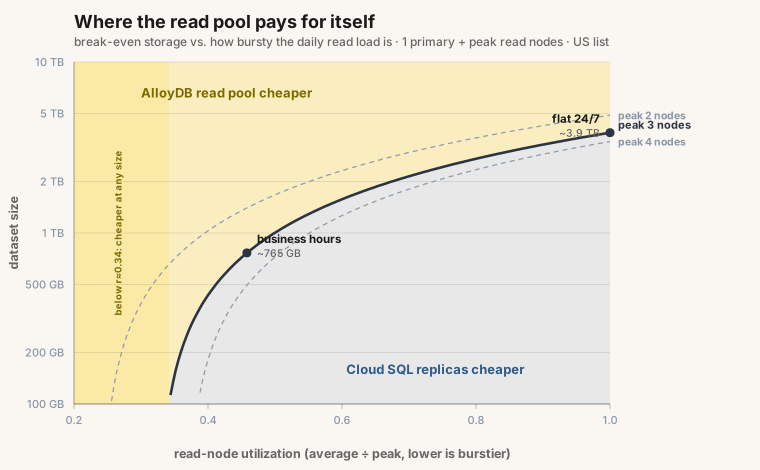
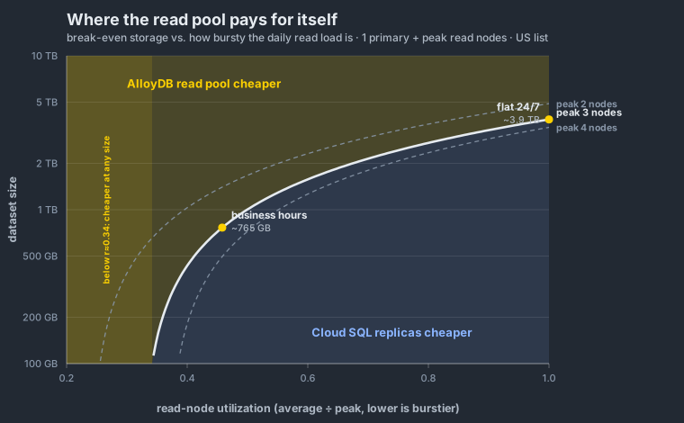
The curve divides the chart in two. Above it, the shared-storage savings exceed AlloyDB's compute premium, making the pool cheaper. Below it, Cloud SQL's cheaper compute still wins. The curve goes up to the right. The flatter your read load is, the more data you need. This is necessary before the storage savings outweigh AlloyDB's compute cost. Your workload is marked on this chart. More terabytes push it up, while a burstier day shifts it left. Both factors move it closer to AlloyDB's side of the line. Below about a third of peak the curve leaves the bottom of the chart entirely, and AlloyDB is cheaper at any size.

AlloyDB automates this process. Its read pool autoscaling adjusts the node count based on CPU usage, a schedule, or both. This means you can activate low-duty-cycle mode as a policy, not through complex scripts. Cloud SQL does not have a similar feature for replica counts.

Two important points apply here. First, when you add a new node, it starts cold. This means it gradually earns its capacity instead of doing it all at once. The buffer cache fills up over a few minutes. During this time, scans that would normally pull from memory must retrieve data from storage. That’s why autoscaling works better for steady reads throughout the business day than for sudden spikes.

Second, the autoscaler adds nodes without shifting existing long-lived connections. If a session opened a connection and keeps it, that connection stays where it is. The new capacity is only used when clients reconnect. AlloyDB’s managed PgBouncer in transaction mode helps with this, spreading new connections across the pool as nodes come and go. Short-lived pooled connections utilize the new nodes, while long-held sessions leave them unused.

So, the recommendation depends on read patterns. If reads are steady all day and data is under a few terabytes, Cloud SQL replicas are more cost-effective. For bursty reads, like business-hour dashboards or nightly reports, AlloyDB’s autoscaling read pool is cheaper and self-scaling.

If your reporting can handle a few seconds of lag, streaming replication is fine. You can skip this section.

AlloyDB AI: the part that's interesting without GCP

Every managed PostgreSQL has pgvector now. AlloyDB stands out because of ScaNN. This is Google’s approximate-nearest-neighbor algorithm. It powers their internal search and comes as a PostgreSQL index access method. It works with pgvector’s `ivfflat` and `hnsw`.

-- pgvector HNSW, available everywhere
CREATE INDEX ON embeddings USING hnsw (embedding vector_cosine_ops);

-- AlloyDB ScaNN (verified on Omni; sq8 quantization keeps the index small)
CREATE INDEX ON embeddings USING scann (embedding cosine)
WITH (num_leaves = 1000, quantizer = 'sq8');
-- query-time recall/latency knob. The LOAD is not optional: without it the SET
-- silently does nothing and the search runs at a shallow default (see below).
LOAD 'alloydb_scann';
SET scann.num_leaves_to_search = N;

-- The query doesn't change; the planner picks the index
SELECT id, content FROM embeddings
ORDER BY embedding <=> '[0.1, 0.2, ...]'
LIMIT 10;

The claim to test is that with tens of millions of vectors, ScaNN maintains high recall while reducing query latency. In contrast, HNSW starts to cost a lot in memory and build time. I ran it at 10M vectors of 1024 dimensions, cosine distance, against exact ground truth. The cost half of that claim holds, and holds convincingly. I couldn't settle the recall half, and the reason is more important than the number.

The half that holds is index size and build time. ScaNN's sq8-quantized index came to 2.6 GB against ivfflat's 76 GB, roughly thirty times smaller, and built in six to seven minutes against fifty-three. Both runs of the harness put the index sizes within a megabyte of each other and ivfflat's build within half a percent; ScaNN's own build time varied more between them, 357 seconds and 437 seconds, so call the build advantage seven to nine times rather than a single figure.

One of the issues that surprised me is query-time setting scann.num_leaves_to_search. It only works if alloydb_scann is loaded first; otherwise, it defaults to a shallow search. Adding the library to shared_preload_libraries causes server restart failures. The only reliable method is loading it per session. My initial 10M run requested a deep search but returned a recall of 0.15, with no indication that the knob was ignored. I won't report the recall figure since my runs disagreed, and the test to clarify this never happened. I’ll focus on ScaNN's claim of maintaining recall at deeper levels, but I trust it the least. Proper testing should plot recall against search depth with your own data; I’d prioritise index size and build time instead.

At the end I didn't manage to get a clean 10M build number for hnsw using this setup. The parallel build hit resource limits. One attempt faced disk issues, while another had a shared-memory segment that was too small. This shows that building a full-precision graph over ten million high-dimensional vectors is costly.

Therefore, the scorecard is shorter than the datasheet and less detailed than I wanted. ScaNN's index excels in size and build time, showcasing solid engineering through a standard PostgreSQL interface. I leave its recall claim open. Both index builds, the ivfflat baseline (76 GB, 53 minutes) and the log of the disrupted run, are in the repo.

ScaNN ships with Omni, so it doesn’t need managed AlloyDB or GCP. The other part of AlloyDB AI, the google_ml_integration extension, which calls Vertex AI models from SQL, does require them.

-- model id is a current Vertex model: text-embedding-005 (English/code, 768d) here;
-- gemini-embedding-001 is the higher-quality, higher-dimension option
SELECT id, google_ml.embedding('text-embedding-005', content) AS vec
FROM documents;

If you're on GCP and already call Vertex, that saves a data round-trip. If you're not, it does nothing for you.

Cross-region: DR, not active-active

AlloyDB allows up to five secondary clusters in different regions. Google reports replication lag in the tens of milliseconds. It looks like cross-region HA, and it is, within one constraint: writes go to the primary region, always. Secondaries are read-only until promoted, and the two promotion paths are not interchangeable.

Failover (DR promotion). The secondary declares itself primary and starts taking writes. Whatever WAL was in flight and unconfirmed when the old primary died is gone. This is the path for "the region is down and we accept the loss window."

Switchover is coordinated. Drain the primary, confirm the secondary is caught up, swap roles. Zero loss, but both sides must participate.

An active-active deployment does not exist.If your architecture requires writes in multiple regions, AlloyDB isn't the solution. The documentation is clear about this. The key risk to avoid is human error. This happens when an operator promotes a system during a minor issue, incurring data loss. A proper switchover would have managed this situation smoothly.

What "fully compatible" actually covers

As already mentioned - "fully compatible with PostgreSQL" means AlloyDB uses the PostgreSQL wire protocol and runs its SQL dialect. psql, libpq, JDBC, psycopg, the ORMs all work, and that's not nothing; it's the difference between migrating and rewriting.

Here is what it does not mean.

AlloyDB is not community PostgreSQL. It’s a Google fork with unique changes, including a columnar engine and planner updates, which aren’t shared with the community. The storage interface is tied to Google’s infrastructure. While Cloud SQL uses upstream PostgreSQL, AlloyDB modifications remain in the fork. AlloyDB matches community releases closely: PostgreSQL 18 reached GA on AlloyDB in May 2026, within months of the community release. Upgrades from older versions are easy, but security and behavioural fixes come solely from Google’s fork.

Extensions are an allowlist, and the allowlist differs between the two products in ways you would not guess. Managed AlloyDB's approved set is generous for the mainstream, and the Omni image ships its own bundle; they are not the same bundle. Compare the Omni Docker image contents (from pg_available_extensions) with the managed supported list.

extension	Omni image	Managed AlloyDB
pg_stat_statements, pg_repack, pg_partman	ships	yes
pgaudit, pg_cron	ships	yes, behind a flag
postgis	not bundled	yes
plv8	ships (3.2.3)	no
timescaledb	not bundled	no
pgvector, hstore, pg_trgm, pgcrypto, uuid-ossp	ships	yes

Two counterintuitive points: plv8 is included in the Omni image but not on the managed allowlist, making "AlloyDB supports plv8" true for Omni and false for managed. Conversely, postgis is supported by managed but not included in Omni, requiring manual installation. "Built for PostgreSQL 18" doesn't guarantee compatibility with AlloyDB Omni 18. timescaledb is unsupported on both.

AlloyDB Omni added Transparent Data Encryption (TDE) in preview (Omni 18.1.0). This feature provides cluster-level at-rest encryption. It also supports keys in external KMS, such as HashiCorp Vault. In contrast, community PostgreSQL lacks built-in TDE, relying instead on filesystem encryption or pgcrypto. Managed AlloyDB uses standard cloud at-rest encryption with Cloud KMS. The Omni feature is important. It adds a debated capability to self-hosted builds. This is similar to the changes seen in the columnar engine and planner.

The config surface is curated too. There is no postgresql.conf and no pg_hba.conf; parameters are exposed (or not) through the GCP console and API, and ALTER SYSTEM is not yours to run. Most teams won’t miss the hidden flags. However, teams that carefully tune PostgreSQL will quickly notice which ones are missing. The storage works similarly: pageinspect, WAL inspection, and anything that deals with the physical format is either removed or has a new meaning. So, you rely on AlloyDB's insights about what happens below the buffer pool.

The version story is a genuine strength, though. AlloyDB tracks new majors fast and ships one-click in-place upgrades, and it keeps old majors alive past community EOL. Both ends of that range are real enterprise value. You are neither forced onto a migration on the community's clock nor stranded on a version the community has dropped.

The fixes for your version, including new-major support and extended-support patches, come from Google. They are for Google's fork since that's the code you are using.

The governance question

This part of the evaluation bothered me the most, and it's the hardest to benchmark. PostgreSQL is more than just source code. It’s a development process. There are public mailing lists for design talks, commit messages that explain choices, and release notes that track changes in behaviour. Plus, there’s a 30-year history that anyone can read. When PostgreSQL surprises you, you can trace back to the thread where the decision was made.

Google does invest in that process, and it is worth being honest about how.

Google shares that it employs key PostgreSQL contributors. Their latest work is open for all to see. This includes:

• Design and review of PostgreSQL 18's native conflict detection for logical replication.
• The long-awaited logical replication of sequences.
• Fixes for core deadlocks and upgrade bugs.
• A spot on the PGConf.dev 2026 program committee.

The contribution stops short of AlloyDB itself, though. A search of the pgsql-hackers archives for "AlloyDB" still returns zero hits, and that is not a quirk of branding. Google's upstream work is standard PostgreSQL. It’s contributed under individual and Google Cloud names, benefiting everyone. The architecture that makes AlloyDB AlloyDB is developed entirely outside that work, and proposed to the community nowhere.

Aurora and Azure's PostgreSQL services are similar. This section applies to both, differing only in serial numbers. Choosing either means selecting a vendor as your database governance authority instead of the PostgreSQL community. This decision should be clearly noted in your architecture decision record.

One observation follows from the architecture itself. The wire protocol is now the only stable boundary. Tools that operate there, like schema introspection via pg_catalog, migration planners, and connection proxies, work the same with AlloyDB. This is because Google has promised to keep that layer stable. Tools that reach below it break. As more of the fleet moves onto wire-compatible-but-divergent engines, the protocol-and-catalog layer is becoming the de facto portability standard, more durable than the "it's PostgreSQL" label, which increasingly just means the PostgreSQL wire protocol.

The community could enhance Mayur's PostgreSQL Compatibility Index, which already exists. The PG Scorecard rates vendors, with AlloyDB scoring about 93%. This score reflects SQL compatibility but doesn't assess the storage engine or operational aspects. The article and score aren't conflicting; they evaluate different layers. What's needed is a matrix for the underlying components, including extension portability and governance transparency. Each engine would have varied scores, and combining both matrices would provide greater insight than either alone. This could be a great topic for a pgConf talk.

When AlloyDB makes sense

Marketing aside, the decision is more tractable than the feature list makes it look.

A good fit comes when:

• You're already on GCP and want the infrastructure chores gone. Failover is seamless since there’s shared storage and no WAL to replay. Storage expands automatically without needing resize windows. Plus, the write path avoids PostgreSQL's full-page-write cost in the managed service. Three concrete wins, and none of them costs you a config knob

• HTAP load allows for fast reporting and analytics on live data. The columnar engine speeds up scans, bypassing the warehouse, while a read pool node separates these from OLTP writes. This combination of quick analytics on the main node and distinct compute on a shared-storage read node is challenging to achieve with standard PostgreSQL.

• Your read-heavy workload needs replica freshness in tens of milliseconds, while a streaming replica can take seconds. You can accept a wider boundary during write bursts. The read pool’s costs work for your needs. If you have multi-terabyte data or bursty reads, you can autoscale down. For flat 24/7 reads under a few terabytes, Cloud SQL remains cheaper, as noted above.

• You want the columnar engine without GCP; that's Omni, knowing it's the query layer only

Not so good fit:

• You depend on extensions off the allowlist: timescaledb, plv8, anything pgrx, anything superuser

• Your tuning, tooling, or debugging relies on upstream PostgreSQL behaviour below the protocol. This includes config access, storage inspection, or WAL tooling.

• Major-version upgrades need to happen on your schedule

• You need active-active across regions

• You're not on GCP and were considering managed AlloyDB; that's GCP-only, and everywhere else means Omni, which is different product (see above)

The columnar engine justifies its memory use when analytical queries scan millions of rows for a few columns. This makes scans faster. However, it doesn't isolate these scans from concurrent writes; that's the read pool's role on a separate node. Use both together. It’s not effective for index-served workloads, point lookups, or small tables in the buffer pool. It can also be expensive for write-heavy tables with pinned columns. See the numbers below for crossover points.

The numbers

TPC-H scale factor 10, median of 5 warm runs, one cold run dropped, all on 8 vCPU / 64 GB in the same region. Times in milliseconds. Two parity gaps are worth naming rather than burying: standard PG is 18.4 while Omni is 17.7, because the Docker image lagged a major at the time, and Omni auto-tunes shared_buffers to about 47 GB where the native instance ran 16 GB. I ran Omni at both sizes to check whether the second one mattered, and it doesn't move anything material: Q6 is 2,592 ms at 16 GB against 2,681 ms at 47 GB. Both gaps are real, both are in the repo, and neither carries the result. The two Omni columns represent the clean experiment. They use the same binary and storage. One has the columnar engine off, while the other has it on.

query	standard PG 18	Omni, engine off	Omni, engine on	managed AlloyDB
Q1	11,969	14,056	10,159	9,922
Q5	2,496	2,374	1,870	1,521
Q6	2,669	2,681	69	62
Q12	2,357	2,909	706	682
Q14	1,293	1,005	555	481
Q18	34,301	29,924	26,168	31,353
point lookup	0.107	0.096	0.119	0.120

Read the two Omni columns across. Q6, a selective scan of a few columns, drops from 2,681 ms to 69 ms, 39x. Q12 drops 4.1x and Q14 1.8x, both joins with date filters. Q1 moves 1.4x because it sums four numeric columns over nearly every row and the arithmetic dominates. Q18, an uncorrelated IN subquery, moves 1.14x, the smallest win in the set. The point lookup stays put: 0.096 ms with the engine off against 0.119 with it on, and at SF100 it goes the other way, 0.15 against 0.11. Both differences are a few hundredths of a millisecond, which is noise on a query this small. The planner uses the b-tree, and the columnar store doesn’t affect the plan.

Managed AlloyDB (engine on) tracks self-managed Omni almost exactly: Q6 62 vs 69 ms, Q12 682 vs 706, Q14 481 vs 555. The columnar engine behaves the same whether Google runs it or you do, which is the confirmation that the result isn't an artifact of one deployment.

This table hides two key points. First, "standard PG 18" is a hand-tuned native instance. Running the same query on Cloud SQL with default settings (work_mem=4MB and two workers per gather) takes 12,436 ms for Q5. This gap is due to a config default, not the engine. It’s the cost that every managed-Postgres comparison faces; it’s noted in the repo as B-stock.

Second, at SF10, the whole dataset fits in RAM for every config. Here, the columnar advantage comes from vectorized execution and skipped columns, since there’s no disk access. At SF100, where the row store spills to disk, Q6's 39x becomes 311x (the plans are in the columnar section above).

The two controls the engine has to not lose:

INSERT throughput. Loading one million rows into lineitem with its columns pinned into the columnar store, versus not: 1,859 ms pinned, 1,842 ms unpinned. About 1% to keep the columnar blocks coherent, at this write rate. A write-hot table taking thousands of INSERTs a second is where that cost grows; this measures the quiet end of it.

Concurrency and HTAP. On Omni, writes with pgbench and a concurrent analytical scan on the same table show a 13.6% drop in write throughput for row store and 13.5% for columnar store. The columnar engine, meant to reduce contention, didn't help because the scanned table was in memory, eliminating disk wait times. Both scans used CPU and memory bandwidth on the same node as the writes, causing the drop.

To prevent analytical scans from affecting OLTP throughput on AlloyDB, route them to a separate read pool node, accepting visibility lag instead of reduced write throughput.

Testing at SF100 with a 600-million-row lineitem revealed that the disk-bound row-store scan reduced write throughput by 16%, while the in-memory columnar scan dropped it by 29%. Columnar scans, though cheaper and CPU-efficient, increased contention by consuming more memory bandwidth on the write node. Thus, physical isolation on separate hardware is necessary for effective resource management. Each configuration's results were based on median values from three 120-second runs, with raw data available in the repo.

Read pool lag. Under a sustained insert load, a two-node read pool trailed the primary by a median of about 60 ms and, across thirty samples, did not climb as the writes continued (raw samples in the repo). The flat-under-sustained-load shape is the finding, not the absolute value. What this run does not cover is a write burst, which Google documents as able to overwhelm a pool's replication, or a head-to-head against Cloud SQL.

Methodology, raw timings, and EXPLAIN ANALYZE output for every number is available at https://github.com/boringSQL/alloydb-evaluation-bench. If a result doesn't reproduce for you, that's a bug in the article; file an issue.

What Google got right, and what it costs

Adaptive autovacuum is a smart scheduler. It speeds up when the instance is idle and slows down when it’s busy. This feature addresses the common issue of vacuum debt in PostgreSQL. It automates tasks that users usually have to tune manually. It does not move the work off the compute node, whatever the pitch implies. It makes the box smart enough that the scheduling stops being your problem.

The read pool model offers a fairer price for read scaling compared to the replica model. This fairness increases as you expand. ScaNN, as an index access method, is robust engineering. It’s available through a standard interface in Omni, without any GCP charges. The team behind this has a deep understanding of PostgreSQL and knows what users can do without.

What it costs is the other half of this post. PostgreSQL in AlloyDB covers the protocol, dialect, and planner's behaviour. Google owns the storage engine, operational model, upgrade schedule, extension surface, and governance.

The boring answer, as always, is to test it against your workload. The TPC-H numbers above show the columnar engine's best case. Even then, two results didn’t match the datasheet. When the heap spilled to disk, enabling the columnar engine increased write contention to 29%, compared to 16% for the row store. Also, ScaNN’s key query-time knob is inactive unless you LOAD the library first. This cost me a ten-million-vector run and yielded only 0.15 recall, with no warning. Both issues took time to discover, and neither is mentioned in any marketing.

Disclaimer

The article hasn’t been reviewed or edited by Google Cloud team. I asked for internal insights but haven’t received them for various reasons. The benchmark repository was developed over an extended period of timeand is managed using Claude Code. My company - Clusterity s.r.o. - have covered all costs related to the benchmarking.

The work on this article spanned between April to August 2026. Preceded by the evaluation of the commercial workloads.